Bayesian Statistics: Approach to Machine Learning

With this short post, I will attempt to explain how Bayesian Statistics (and stat. as a whole) offers us a powerful lense through which to view machine learning problems.

Bayes Formula

Fundamentally, Bayes wrote about how to update ones beliefs when given new information.

Lets start with a simple example:

From prior experience, there is a 90% chance that men have short hair, and a 20% chance that women do. We see someone, but can
only see there hair, which is short. What is the chance that they are male?

Well, intuitively it is 90%/20%+90% = ~81%.

However, we are presented with new information: we are in a country with 80% women. Obviously, we would need to update our beliefs- and Bayes gives us a way to do so:

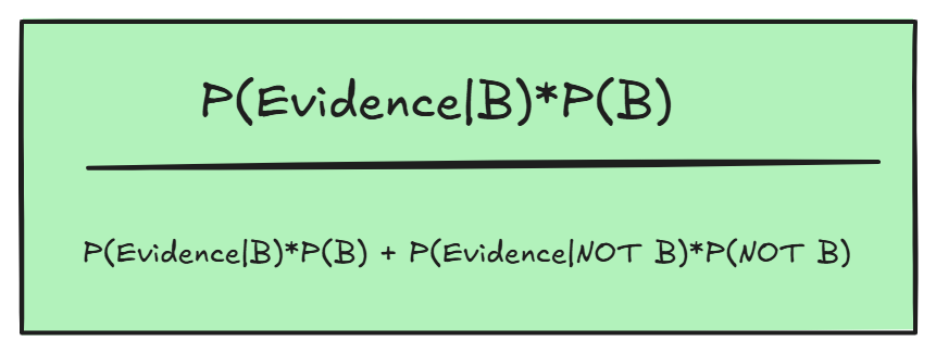
This formula is basically saying: the new probability is (original) belief given evidence, which was our original belief times the proportion of males in the country, divided by the total new probability (the belief given evidence and the chance its not belief given new evidence).

In this case, the evidence would shrink the proportion of the belief (which we would multiply by 0.2) to the overall whole (multiply NOT B by 0.8, given the new information).

Here is a geometric interpretation:

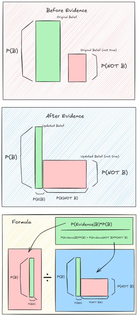
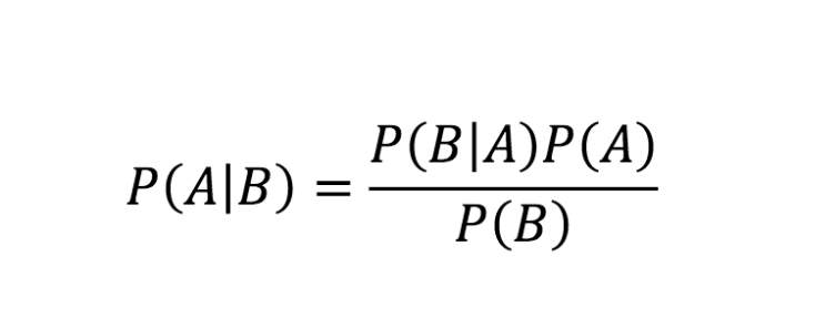
The multiplication, and overall method has a clear geometric interpretation and is very intuitive.

If you do not fully understand how this relates to probability and statistics, we will go into this in-depth later in the section asking the question:

How does this approach of ‘updating our beliefs’ apply to real problems?

Frequentist vs. Bayesian Approach to statistics

Statistics

Humans have always had some data and wanted to learn from it. This is the fundamental reason for statistics. But we need models of our data that are non-deterministic: we need to say how certain or uncertain we are about an event happening, given data.

Statisticians therefore model the distribution of data with PDF’s (probability distribution functions). While real, naturally occurring PDF’s are often influenced by an infinite number of factors and very complex, we can use ‘parametrized’ PDF’s (such as the normal distribution) which only have a few variables(parameters), and can model a variety of frequently-occurring probabilities in the real world.

For example, we can train a machine learning model to estimate the PDF of heights in a population by training it to tweak parameters for a selected parametric family (which would be mew and sigma for a normal distribution). Then, we can infer about the probability for novel data! This is called statistical inference.

Bayesian vs. Frequentist approach to statistical inference

Baye’s theorem is simple, but it ushered in a new era of thinking about probabilities in a subjective way (Bayesian statistics), rather than as objective truth (Frequentist statistics).

So, what is the difference between these two approaches to statistics?

• Frequentist probability is saying that probability is just frequency. For example, the probability of rolling a 2 for a dice is based on data collected over many samples. They believe that there is an underlying probability, but it only shows itself as we get a huge number of samples. For any given event, they would say that there is no probability. Probability only manifest itself as we collect many samples, and the more samples we get, the more accurately we can guess the true underlying probability, which is the same for everyone.

The problem with a frequentist approach, is it assumes we can repeat experiments, and collect a large number of samples to approximate the true probability.

• Bayesian statistics, as we saw previously, involves updating our beliefs based on evidence collected, and believing that there is inherent uncertainty in our understanding (parameters) of the distribution of our data. For example, we have a prior belief p(rolling 2), and we assume it to be 1/6. As we get new information (for example, that 100 6’s were rolled out of 200), we update our belief accordingly. But probability is also subjective: if someone where to think that our dice was biased, they would have a different prior belief, which would result in different interpretation of the evidence (although with more evidence, the beliefs would converge).

A problem with this Bayesian approach, as we will see, is that based on our prior, we will get different results (subjective nature), which is not a problem with frequentist approaches (probability is an underlying truth).

Interestingly, Laplace (the one who popularized Bayesian statistics) did not believe in the existence of uncertainty. Therefore, he believed that there are no underlying distributions, just subjective ignorance, and therefore subjective probability distributions.

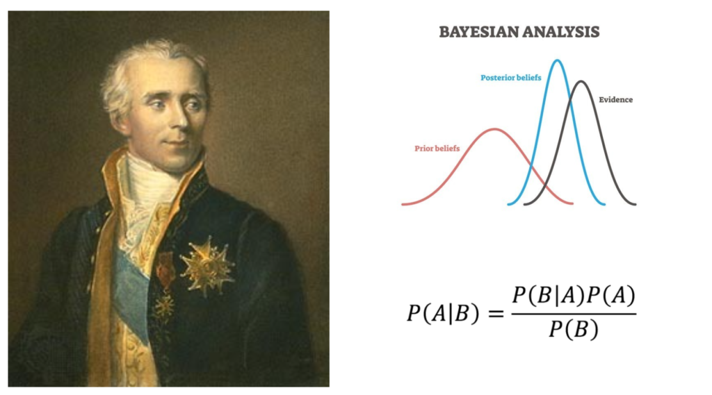
Here’s a simple example:

If we flip a coin, and you ask a Bayesian the probability, they will
say 50%. Then after they see the coin land, they will update their belief based on the outcome. If you ask a frequentist, they will say that there is no inherent probability, but that if you do 10,000 experiments, a probability will manifest over the many examples revealing an approximate of the true distribution.

Now, here’s an example using simple parameterized distributions. Remember that these allow us to model probabilities for complex events. In this case we will only be dealing with a binomial distribution (yes/no outcomes).

I want to find the probability that a bike that I am looking to buy will break in 5 years. I will feel confident that it won’t break if I know there is a 95% probability that it doesn’t. The data says that out of 200 bikes, 210 lasted over 5 years.

Frequentist Approach to Bike Problem

We have 210 experiments, and 200 are positive. Therefore, we have an estimate of the ideal probability (given infinite experiments): 200/210 (95%). So our binomial distribution’s one parameter is 0.95. However we cannot be too sure of this parameter, because we did not have infinite samples; so we need to run a confidence test to see how likely this probability would be given more samples. We are testing against our null hypothesis which gives us information about whether our sampling was statistically significant, or the probability our 0.95 parameter was not completely random.

Our p-value gives us this. It is the probability that we get at least the same extreme results given that we were randomly sampling. For example, if we have a high p-value, there is a high likelihood that our null hypothesis is true, because some completely random sampling would have a high probability to generate our results.

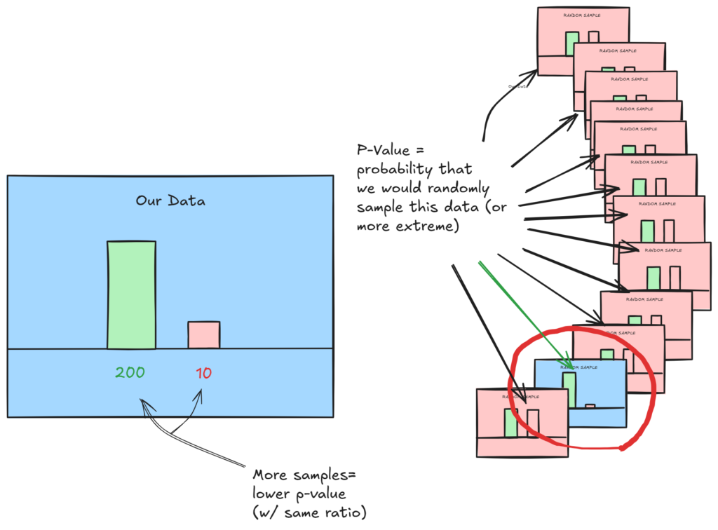
A low p-value tells us our data is not likely to come from random sampling. In this case, our ‘(null) hypothesized probability’ was 0.5. If it where higher, it would be more likely we could sample this, and the p-value would be higher. But for now, we’ll stick with random.

Our p-value generated in this case is essentially 0: it would be very unlikely to get our sample randomly.

Another frequentist tool we can use is our ‘confidence interval’. This tells us, for a given probability, the range that our gathered data could lie. For example with a 95% confidence level, we would find the most extreme values that would encompass exactly 95% of estimated probabilities for future experiments.

Our confidence interval is 0.91417 ≤ p ≤ 0.97693, which tells us that 95% of future repeated experiments will lie in this range.

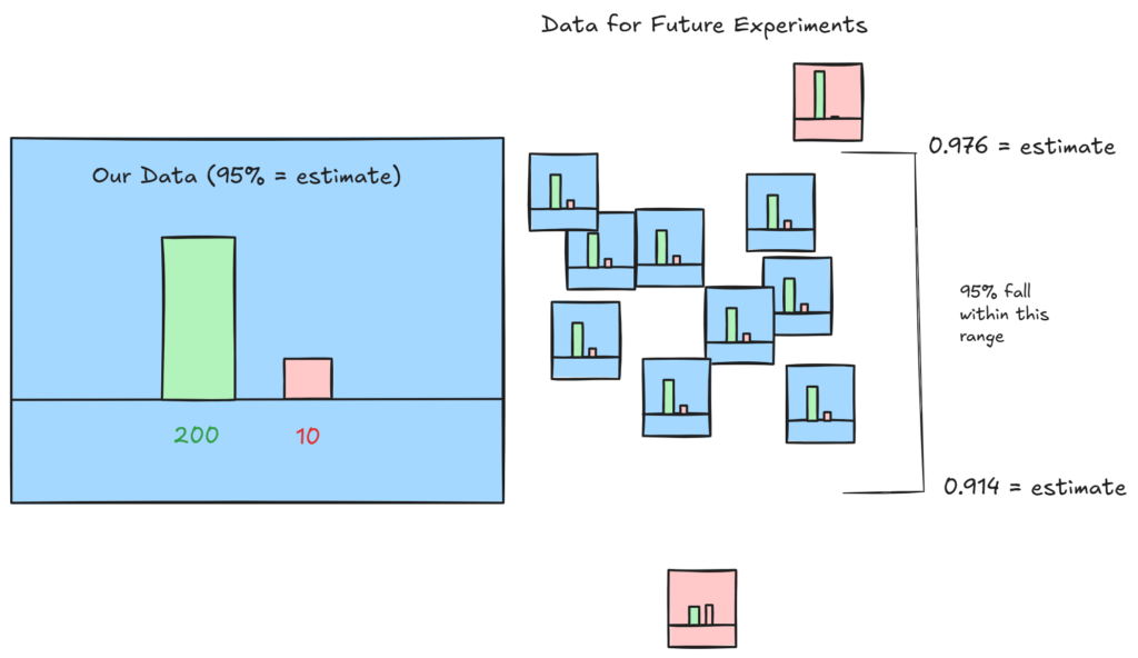
So, we have calculated how likely our results would have been to be randomly selected, the confidence interval for future experiments, and found an estimate for the probability: 95%.

Throughout this approach, we operated under the assumption that there was some true underlying parameter value (probability distribution), and that to get it we just needed more samples. Our p-value and confidence interval quantified how much uncertainty our parameter carried (and are inversely proportional to sample size), given that we didn’t have infinite samples.

It is clear how the frequentist approach is both objective, and reliant on many samples to achieve a close-to-reality view of uncertainty.

We would follow a similar approach if we wanted to model the parameters of a more complex, or continuous distribution such as a normal distribution.

Bayesian Approach to problem

To begin, Baye’s theorem isn’t necessarily Bayesian, rather, how it’s used as an approach to modeling probability is Bayesian. When we first talked about using Baye’s theorem we declared a single prior (90%), however in a Bayesian approach, the prior is said to be a probability distribution (because we are uncertain about it) that we update given new evidence).

This is the most important thing to understand: our parameters θ that define our function p(x|θ) (probability of x given the parametric function) will take on continuous values, reflecting our uncertainty (or ignorance) of the underlying distribution.

This makes things a little more complicated, as we will be dealing with two probability distributions: p(x|θ) and p(θ). Lets look at how we would solve this problem with Bayesian inference:

First we must choose our prior, p(θ), which is the ‘subjectivity’ which will be influenced by our data as we collect it.

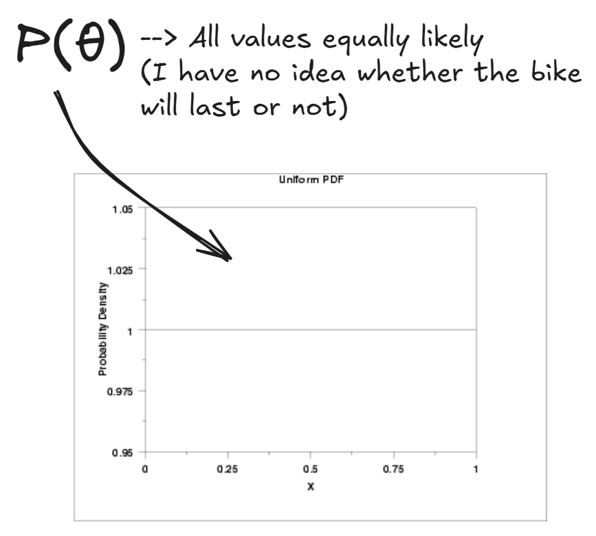
We choose a uniform distribution for our value of theta: we have no idea whether the bike will last, so we assign equal probabilities for all values. (This distribution is actually a parameterized beta distribution, more on that later)

So now lets take a look at the rest of Baye’s formula, and see how it can be used to update our prior beleif of p(θ) given our data:

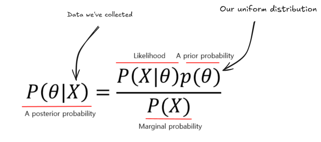
Ok, so remember that the data we collected was 200/210 bikes last more than 5 years. Now, how do we update our prior θ given this information?

Well, Bayes formula tells us that by multiplying our prior by our p(X=data|θ) and dividing by p(X) will give us our new prior. Here’s what that is saying:

1. Our new posterior probability for theta will be proportional to how likely X was given our prior theta, times our prior theta. (basically, the parts that made X likely, we grow, and the other parts we shrink.)
2. We divide by p(X), which is the overall probability of X given theta was not true and theta was true (this is just a number that we get).

To approach calculating p(X|θ) in an intuitive way, let’s pretend we drew from θ’s distribution 1 million times, and counted how many times we replicated our results for each random θ we sample. We will discretize our P(θ) distribution as to be able to approximate with this method.

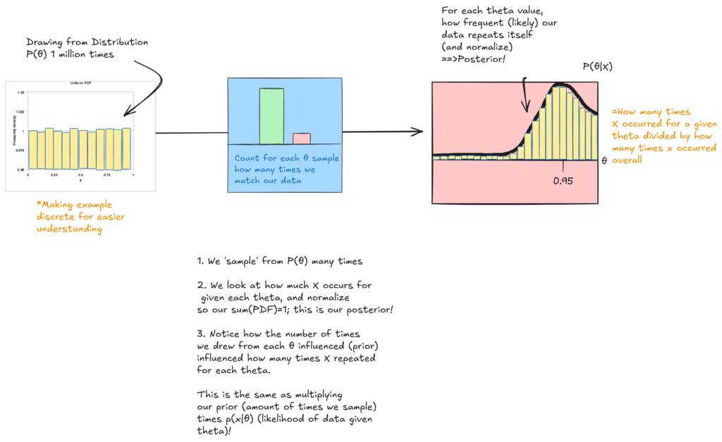
And this is our posterior probability! Hopefully this process of sampling from a prior distribution to try to reproduce our data gave you an intuition for why P(θ|X) is proportional to P(θ) and P(X|θ).

But sampling sometimes is not plausible, as it requires a lot of computation, so we may be able to actually model the likelihood of our data P(X|θ) as a function and multiply it with our continuous distribution (given that we chose a simple prior distribution). In general, the likelihood of our data is:

which means the probability assigned to each data point multiplied at all data points. However, we need to calculate this not for one θ, but for all thetas (to get p(X|θ) distribution).

To do this, we need a likelihood function. Luckily, because we choose from a common parametric family (binomial distribution) we have this function for the likelihood of a binomial distribution given parameters:

Given this function, we can graph it for all θ, and then multiply it by p(θ) to obtain our posterior (and normalize afterwards). Since θ is uniform, we don’t have to do anything to the function P(X|θ) (including normalization), and therefore, we just graph our evidence and get our posterior P(θ|X)

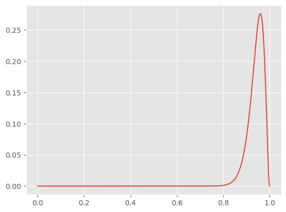
Now, we have an updated posterior distribution for θ! This models our current level of certainty in our predictions, and its easy to infer that with more data we’d be more certain (given that this is literally just the binomial distribution).

We can do better than confidence intervals now, and say the probability that theta will lie within a specific region ∫p(θ|X).

Choosing priors, and Conjugates

In this simple problem we were only dealing with two discrete outcomes, and therefore our distribution p(X|θ) was a simple binomial one, and we were able to parameterize p(θ) with a beta distribution. Due to the mathematical properties of the distributions, we didn’t have to worry at all about approximating p(X|θ), or the marginal p(X), we updated our prior based on the formula for updating a beta distributions prior.

There when our posterior is the same as our prior, we refer to this as a conjugate prior. Many common distributions (exponential, Gaussian) also have this great property of being conjugate for certain problems. For example, the beta distribution is the conjugate prior for binomial distributions, geometric distributions and others, but not for most other cases (where there aren’t discrete outcomes).

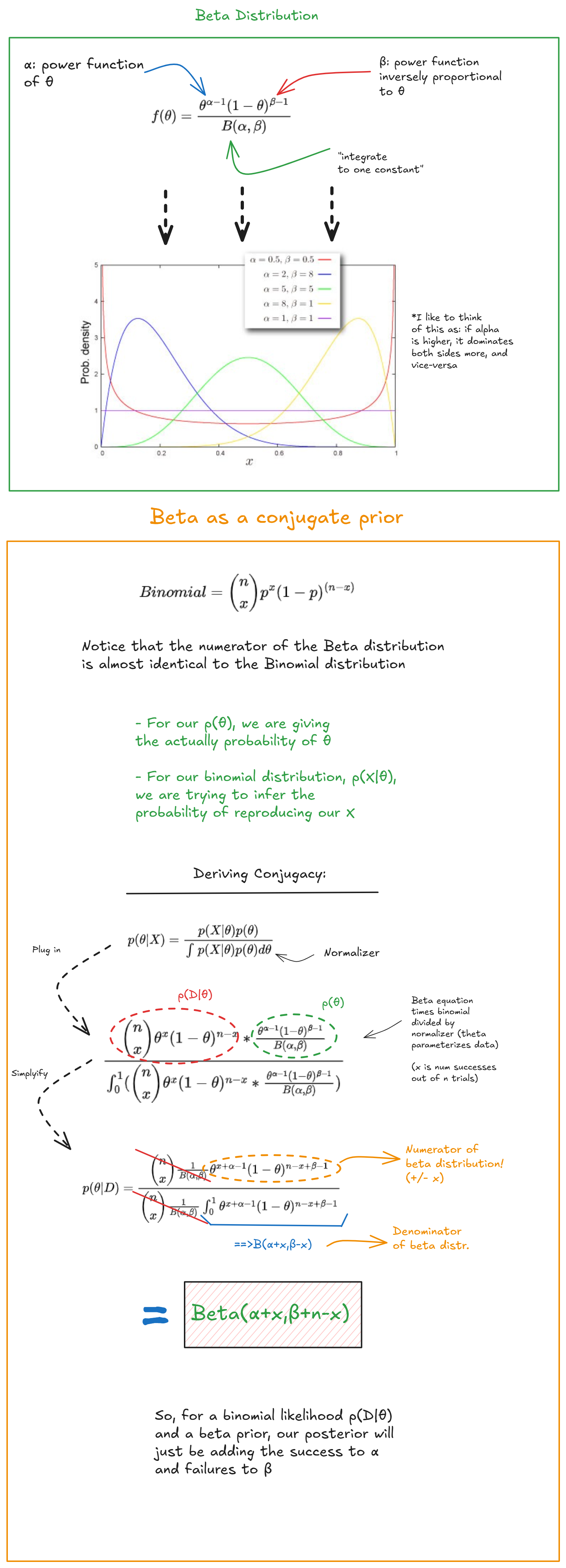
There are other examples of priors that behave nicely under certain likelihood PDF’s: for example, if we parameterize the priors for mu and sigma in the right way, we can obtain conjugate posteriors for both.

However, this is assuming we’ll be working with low-dimensional data and working with few priors. For more complex examples, we’ll actually need to revert back to the previous prior-sampling method, but this time we’ll be sampling from the joint distribution of our many priors, and using algorithms to optimize this sampling in parameter-space. We’ll explain this in-depth in the next section.

Maximum a posteriori estimation

For a final word on interpretation of our Bayesian analysis we preformed in getting our posterior p(θ|X), we will talk ab

Previously, we briefly discussed MLE estimates, which is maximizing the likelihood of our data p(X|θ), assuming theta is a fixed value. Linear regression is an example of this, because we iteratively maximize p(X|θ) for our entire dataset by making our line closer to the points. We could do the same iterative process with, for example, a normal distribution and some data.

Switching to a Bayesian perspective, Maximum a posteriori, or MAP, is about finding the best single θ value for our posterior distribution. Compared to MLE, instead of maximizing p(X|θ), we maximize p(X|θ)p(θ); we are basically optimizing the same thing, just factoring in our prior (and ignoring the marginal, which is constant for varying θ).

In practice, we will maximize the log-likelihood of theta, because maximizing the log is the same as maximizing the value itself, and it is easier to work with.

Working in higher dimensions

Now that we have an understanding of a Bayesian approach to statistical inference, it is important to note one more time that we will be dealing with high-dimensional data that does not have closed-form solutions or conjugate posteriors.

The above equation is maximizable because the marginal (denominator) does not depend on the specific value of theta we choose, however in the future when we want to calculate the posterior, the integral in the marginal will almost always be a problem, since for more than 1 prior:

So, we would treat our z’s (parameters) as jointly distributed, independent priors, and then multiply this PDF by X’s likelihood PDF. Then, we would integrate over all n z’s, which would be infeasible, since for each z the integral would grow exponentially.

Clearly, sampling might be to our advantage in this case again. We will now discuss ways to effectively sample in high-dimensional space from our priors to obtain posteriors, and other ways to approximate posteriors.

Applying to Machine Learning

So far we’ve discussed simple examples to try to build our intuition for Bayesian and other statistical methods, and in this section we’ll see how we can apply this thinking to more complex and real-world problems involving machine learning.

Here I will attempt to gather and understand the machine learning techniques that adopt Bayesian and statistical approaches to solving problems.

Linear Regression

Let’s warm-up our Bayesian thinking by going through Linear Regression through a Bayesian point of view.

Typically we try to fit some data with n different weights, and find the best weights that minimizes mean squared error, and potentially some other regularization.

However, we can approach the problem from a Bayesian point of view as follows:

Similar to MLE, or just maximizing the likelihood without a prior, we are trying to minimize the MSE loss. However, it is interesting to note that maximizing our posterior also forces us to account for our prior’s distribution; specifically, we cannot stray too far from it, and it inherently adds L2 regularization. This reveals how when approaching something from a Bayesian perspective we can gain new insight into our problem.

Markov Chain Monte Carlo

Before we go into the details of this strategy, let’s review what we did in Linear Regression, and generalize it to more advanced machine learning models.

1. We have a dataset X
2. We have a model (usually neural networks) to give probabilities for X, so these can be seen as assigning a PDF to X
3. We want to infer the parameters of this model p(θ|X), given our data (similar to what we did in linear regression, just more parameters).
4. We do this by maximizing the likelihood and the prior distribution.
5. Sometimes, there are some hidden, or latent, variables we would like to model. (more on this later)

Now we will begin to talk about how to estimate probability distributions when directly solving them is not possible.

Markov chain Monte Carlo is a powerful method that we can use to approximate our posterior distribution when we cannot evaluate the marginal through integration.

1. Sampling (Monte Carlo)

‘Vanilla’ Monte Carlo integration, is simply randomly sampling from an area, taking the average of that sample, and then multiplying by the volume (or area) of the domain we sampled over. This, however, is not fit for our problem, so we will not discuss it further.

When we sample from a distribution and have a way to evaluate the likelihood at a given point (IE our posterior numerator), but not a way to evaluate the overall function, we can sample from another distribution, such as the normal distribution, and then accept/reject samples that we ‘propose’ in order to make them match our target distribution.

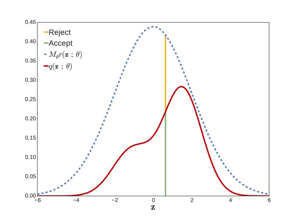
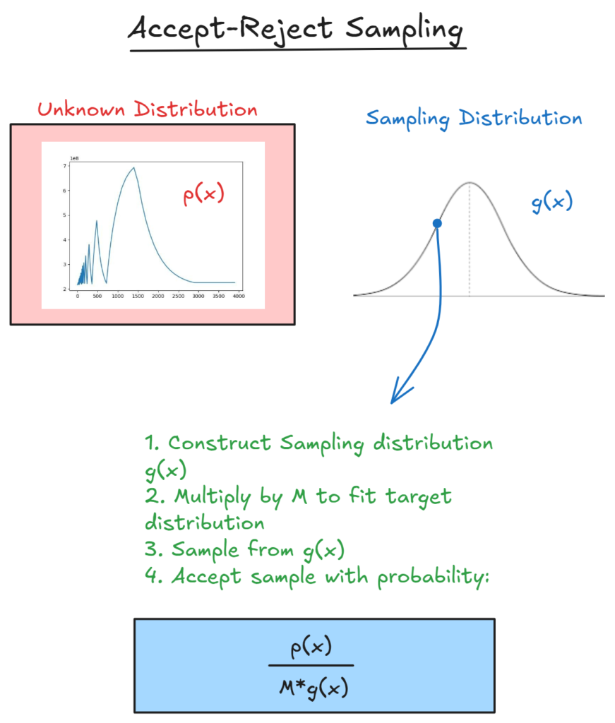
this ensures that the probability we draw a given sample matches p(x).

However, this is a slow method, and there are much better ways to do this, as we will see below.

2. Markov Chains

Markov chains are simply systems in which the next state is only dependent on the previous state. Here is a simple example:

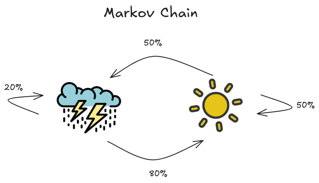
As we can see, each probability p(state_n) only depends on p(state_n-1), which the essential property of Markov chains.

Another useful part of these Markov chains, is over time, the proportion of the number of days being cloudy versus sunny will converge. This makes sense, because we know the probabilities for each given state transition, and we can simply add these up to get our overall probabilities:

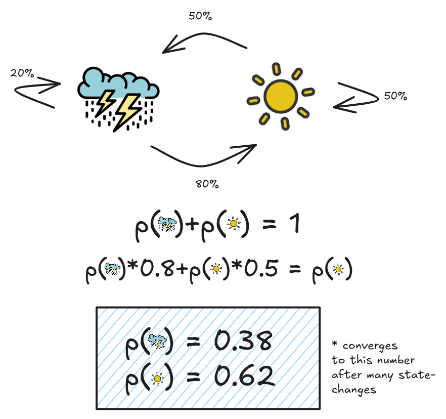
While you can think about why this happens in many different ways, just understand that states with higher probabilities attached to them will be proportionally more likely.

Furthermore, systems with even more states have this same property, and it basically means that over time the states will converge to one given probability distribution.

Markov Chain Monte Carlo

Now, we can put these two methods together to arrive at something that can approximate a distribution p(x) efficiently.

Our goal is to sample with a Markov Chain, that has a steady-state that converges to our desired probability distribution p(x). As long as we have a way to evaluate the numerator of our posterior (p(θ)p(x|θ)) at individual points, we can run this MCMC algorithm and we will be guaranteed a sample distribution that matches our desired (posterior) distribution (over time).

Below I will illustrate the Metropolis-Hastings MCMC flavor, here is a great explanation to follow for further information.

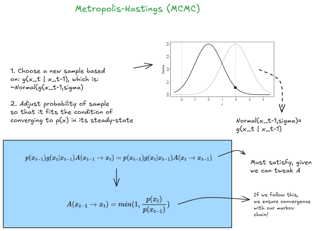
I will not cover the algebraic steps, but essentially we are sampling our proposed values based on the previous sample, and then weighing the acceptance probability in a way that will give us exactly the probability for our Markov-chain to converge and match p(x). And we do this with only needing to know how to evaluate our numerator.

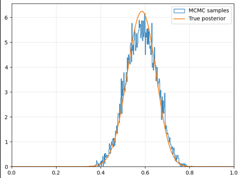
Here is the code I wrote to implement this method, but the strategy is pretty straight forward: just ensuring we achieve a Markov chain who’s steady-state is equal to the probability of our actual distribution.

Application

Now that we are able to generate samples from our posterior, we can evaluate the expected value of theta, the variance, and learn other things that we couldn’t have previously if we lacked a closed-form solution.

Variational Inference

Now, we will be dealing with a technique useful for real-world approaches to modeling high-dimensional data. Variational inference is used to approximate the posterior of latent variables Z with a machine learning model. We will explain this below:

Problem

We start with a dataset X that we observe D from (our data). With variational inference, we are assuming that some hidden variables Z where sampled first, and X is just a realization (projection) of those hidden variables.

However, we cannot observe Z, so therefore:

1. We can try to model p(x|z), or a projection of x for any z
2. We can define a prior for each z: p(z)
3. Lastly, we would like our posterior p(z|x)

Here is a simple illustration:

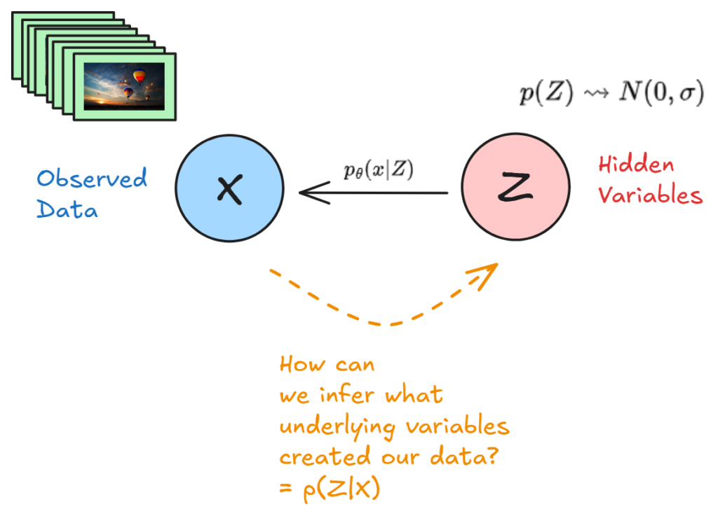
Basically, we have observed some data X, and we would like a model to both map some hidden variables to output a probability for x, and we would also like to know the corresponding posterior p(z|x) given our mapping p(x|z) and our prior p(z).

So, we have 2 tasks here:

1. Find p(Z|x), a way to preform variational inference on our Z variables with a prior
2. Make our models parameters θ maximize the likelihood of p(x|z), our observed data (have a good model of our data)

You may have already thought: clearly, our solution (to posterior inference) is using Bayes theorem! However, Bayes theorem in this case is intractable, and comes with some other problems:

• We would have to compute p(z|x) for every single observed sample
• We can simply not compute p(z|x), because the denominator is intractable

Therefore, we need a ‘surrogate’ distribution q(z|x) parameterized by Φ, where Φ are learned parameters, that we can work with better in order to preform inference on our posterior.

They key part of variational inference is framing this approximation as an optimization problem, specifically: we try to derive an equation to maximize the evidence (model output) p(x) for our model and data, while minimizing the difference between our surrogate q, and the true latent distribution p(z|x).

While at first this may seem intimidating, it basically breaks down into mathematically explaining how we can:

1. Maximize the ‘evidence’ of our model p(x) through reconstruction
2. Minimize the KL divergence between p (prior we set) and q

This intuitively makes sense: we want our model to adhere to our original distribution p(z), while also maximizing the likelihood of the observed data.

This loss formula will be key in our VAE’s, as it allows us to only focus on minimizing the KL divergence, and maximizing the evidence, a problem that can be easily solved with a neural network.

Variational Auto-Encoders

Variational auto-encoders are just an ingenious application of variational inference, that parameterizes the approximation of q(z|x) and p(x|z) with an auto-encoder neural network. q is amortized, or we have parameters that can output a q(z|x) for any x, which is key for our model.

Traditional Auto-Encoders

Auto-encoders are simply neural networks that compress data, and attempt to reconstruct the lower-dimensional compression. The network will usually be somewhat symmetric, and have an encoder that learns a way to encode high-dimensional data to lower-dimensional vectors, and then a decoder which attempts to reconstruct the image.

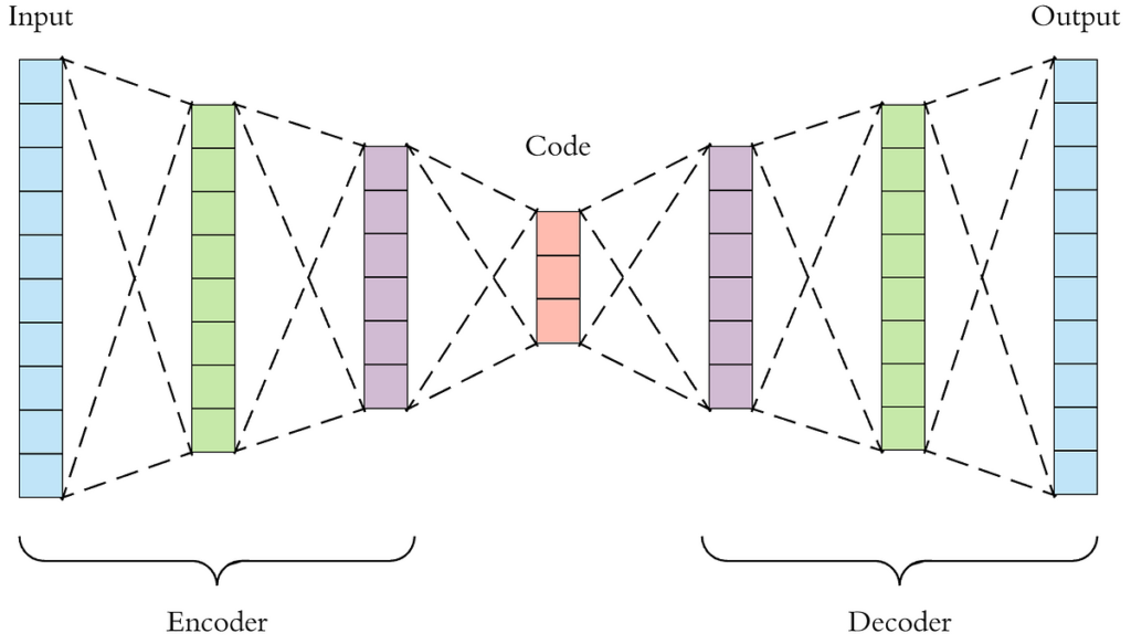
The problem with traditional auto-encoders is that we cannot sample (plug in likely values to our decoder) from the lower-dimensional latent-space, since the neural network is simply trying to reconstruct the image. We do not force it to have any ‘structure’ in the latent-space, and therefore, we have no way to infer what to sample from.

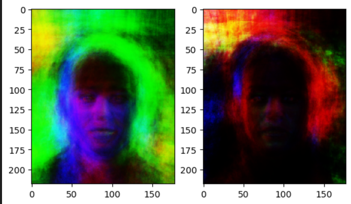
The paper that introduced VAE’s proposed a way to structure the latent space using statistical methods:

1. We set a prior p(z) for our latent distribution
2. We build a model to learn a surrogate for p(z|x), and learn p(x|z), as follows:

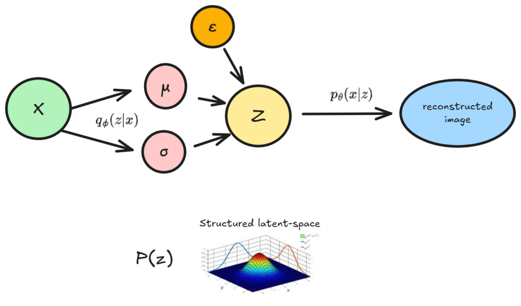
What we are doing here is actually very simple. First, our model learns how to map any x, to any mew and sigma vector, which parameterizes z. Then, we sample from Z (with ε for backpropagation), and reconstruct our image. The only difference between this VAE, and a vanilla auto-encoder, is that we sample from a probability distribution Z, and we also constrain it.

Thinking back to our ELBO in variational inference, we can derive this formula for optimizing the ELBO that fits our problem:

I will not go into the full derivation, as to my understanding the VAE was not discovered through derivation of a loss function, but rather the idea was vaguely motivated by a statistical approach, and then it was theoretically verified.

However, this gives us a powerful tool to optimize:

1. Minimize the KL divergence through minimizing mu, and keeping sigma close to 1
2. Maximize the Average reconstruction similarity p(x|z)

Here is a VAE implemented in code, let’s explore the results, and try to explain why the VAE architecture is doing what it is.

Interpreting Results

Now, let’s move away from theoretical mathematics, and talk about what our model is actually doing.

The first vanilla-autoencoder is simply trained to reconstruct and encoder a latent-vector. Our latent space will look something like this:

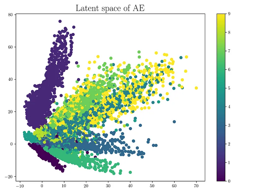
Where different colors are different classes. While there is some overlap, the space is clearly unstructured:

1. We cannot interpolate between classes
2. There is no one region that is more probable than another.

This is a problem if we would want to sample from our latent-space. For example, if we wanted to sample half-way in between a dog and cat image: we wouldn’t be able to do this. However, our variational autoencoder solves this:

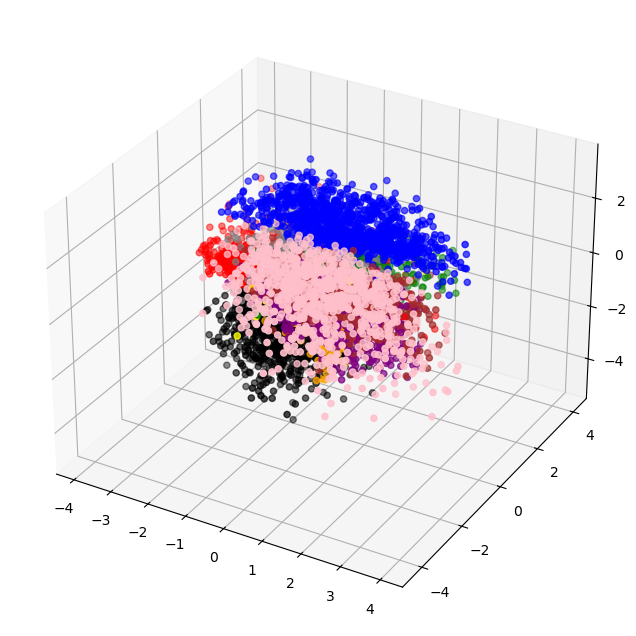
With a steady latent-space, we could clearly sample between classes, and arrive at a probable-image.

This is because:

1. Our model learns to constrain most images near mean zero, so it is forced to use as little expression as possible represent the image. This means similar images will benefit from having similar latent-spaces, and images will share features in the latent space.

2. Our model must be able to account for the reparameterization which introduces randomness. Along with the shared-features, this allows for ‘smoothness’ in the space, or our model is used to accounting for random changes in latent vectors, and still can output reasonable things.

Let’s dig into the model further and see what we can find out about it while sampling from the latent space, and encoding images:

Final Thoughts/Takeaways

I began this article already with a knowledge of how to implement VAE’s in code, and they seemed pretty intuitive. However, trying to read the paper I was completely overwhelmed, and did not understand the notation whatsoever.

I tried to delve into Bayesian statistics, and some of the notation is more, familiar, but I don’t feel I understand the VAE model much better, but I have learned some things:

1. The motivation for VAE’s and most DL architecture’s can be connected to mathematical theories that may be unrelated to the actual conceptualization of the architecture.
2. These theories are not necessary to understand and build with these models.
3. The mathematical motivations behind models can be borderline useless; models should be simple to understand, and a deep theoretical background shouldn’t be necessary.

So here are my parting thoughts, and the main thing I have taken away from this brief foray into statistics to try to understand the model

1. Don’t go in too over your head trying to understand things when there is a clear ‘abstraction’ gap. The people who are writing about it are not inherently better, they are just more fluent in the language, because they have spent more time speaking it.
2. Therefore, do things that you find meaningful, elegant, and can understand (this doesn’t mean don’t push and challenge yourself, but just do so in a way that is meaningful for you)
3. Value understanding deeply and learning over knowing some cool notations (although occasionally they may be necessary)

This was by no means a comprehensive educational resource, and there are undoubtedly many flaws.

Email me: garrishc@ufl.edu for questions, thanks if you made it this far 🙂

Sources

• Auto-Encoding Variational Bayes
• intro to Bayesian data analysis
• Closed form Bayesian Inference for Binomial distributions
• MCMC Duke