Math Behind diffusion models

Here are my notes about me trying to understand the motivations/maths behind DDPM’s, and intuitively why they work, to try to make it feel like we could have invented them! Then, we’ll build it from scratch 🙂

Understanding Log:

11/15/24:

The mathematics to me right now feels very vague and arbitrary!

Starting to understand/ connect dots of why we use ELBO in the context of latent-variable models (and what we are working with in our problem), still not sure 100% about the formulas and how it relates to the optimization objective

11/16/24

I feel progress slowly going through, and trying to understand the derivation of the ELBO, and what it actually means in the context of what we are trying to solve.

Sources:

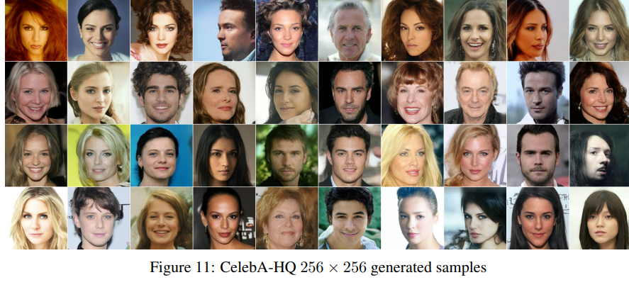
Latent-Variable Models

Latent variables are the low-dimensional projections that we assume to be underlying data (images in our case). With latent variable models, we seek to infer the distribution of underlying latent variables from samples, while maximizing the likelihood our model assigns to the data.

Say we define a neural network p(x|z) which assigns a probability vector x for any latent-vector z. We can define the probability of our latent-variables as p(z), and can make this a normal distribution. Then, we simply need to evaluate:

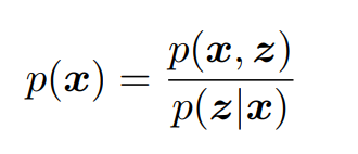
or,

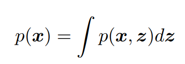
However, we do not have the distribution p(z|x), and we cannot simply initialize or infer it (this is the ground truth). Furthermore, we cannot evaluate the integral, as it would involve integrating over every dimension of z, which is probably not possible!

The reason we want p(x), is because we’ll need to maximize it to obtain a model that has ‘learned’ something about the world.

ELBO

The ELBO (evidence lower-bound), is as its name suggests a ‘lower-bound’ for the evidence. This is exactly what we need: some proxy equation that we can maximize, that will also result in maximizing our p(x), even when we cannot directly do so.

We first introduce an approximate distribution q, which is parameterized by our neural network, and learns a distribution q(z|x) for any sample x, that should be close to the ground truth p(z|x), or the posterior distribution for z given x.

This doesn’t reveal much, let’s derive the equation to see why we might want to optimize this objective:

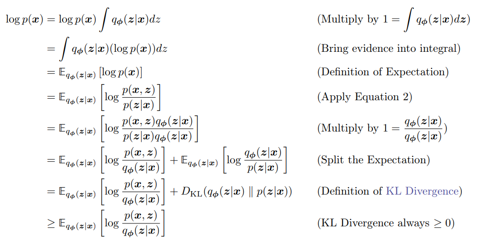
Ok, so through the derivation, we get a more complete picture. KL divergence is always greater or equal to zero, so this is what makes it a ‘lower-bound’ for our evidence (always less than). Furthermore, the ELBO looks a lot like our the equation that we applied in the 4th line, which means we are trying to maximize reconstruction loss.

I like to try to think of this as introducing some new (approximate) distribution, and finding that the distance between the new distribution and the ‘ground-truth’, is how far away we will be from our true evidence (when we use the approximate in its place).

This is a powerful tool, as now we have effectively turned our problem into an optimization with an approximate distribution.

Maximizing the equation:

When we ‘set’ our p(x|z) and p(z), or our generative model, p(x) is necessarily fixed with respect to the approximate distribution q (our approximate is not involved in computing this ground-truth).

So, as we can see in our equation if we maximize our ELBO, we inherently bring the KL divergence down, because they have to sum to log p(X), which doesn’t change. Therefore, the ‘closer’ our ELBO gets to p(x), the lower the KL divergence, given that we are changing φ. Then once we lower the distance (KL divergence) from the ELBO and the true evidence, we can test our model on new samples with the ELBO.

VAEs

Interestingly, if we expand out our ELBO even more, we can obtain:

So, we can split our ELBO up into two very convenient terms:

The first term is our reconstruction loss given our surrogate, it is saying: what do we expect from our p(x|z), given that we model the probabilities of z with q
The second term is simply the prior’s difference with our surrogate!

My interpretation of this, is that in order for q to be a good approximate of p(z|x), not only must it factor in the likelihood of p(x|z), but it must also stay close to the prior. We can try to get q to be arbitrarily close to this, but it will never be as close as p(z|x), which perfectly factors in this balance (given ELBO is a lower bound).

This is because of Bayes theorem:

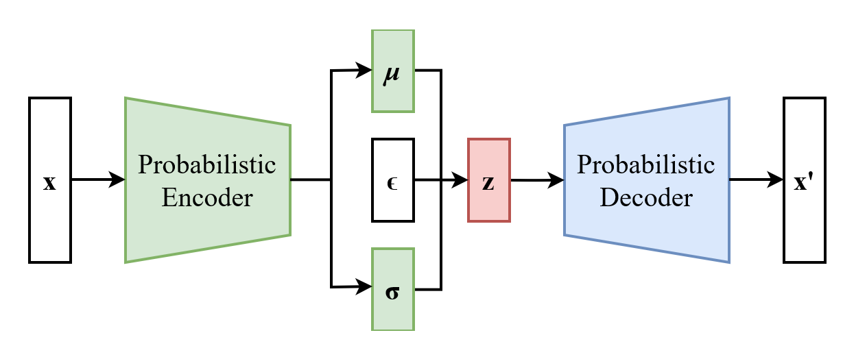
Variational Autoencoders are variational, because they maximize the function q with parameters φ, and they use an auto-encoder structure to do so. Specifically, φ is a neural network that encodes a sample x into a distribution for our latent-vector, and p(x|z) is a decoder neural network that reconstructs our image from a sampled z (from our distribution).

ELBO gives us the tools to solve this problem: since we have an objective to minimize our KL divergence, we can simply focus on minimizing the reconstruction loss for every given sample, and do this stochastically with gradient descent (estimation for the whole dataset). Furthermore, we account for our prior with a KL divergence term in our loss.

Our encoder is q(z|x) with parameters φ, that assigns mu and sigma vectors for any x
Our decoder (generative model) is p(z|x), which deterministically computes x given any z (which works in practice, because we are doing stochastic gradient descent)

Above is how we mathematically define our distributions (no relation between dimensions of latent-variables is assumed).

We can write our reconstruction loss as:

We could compute our KL divergence analytically since we are working with Gaussians, and we would have to use Monte Carlo sampling from our distribution q(z|x) to approximate p(x|z).

Since we cannot compute the gradient of a randomly sampled z^(l) as we see in our function, we sample from a normal distribution, and simply re-scale this sample by the mean and standard deviation provided by q(z|x), which is the same thing, but allows us to take the derivative:

To summarize, we’ve derived the ELBO to try to bring our surrogate distribution close to the actual p(z|x) distribution, and then we try to maximize both the ELBO through φ, and the evidence through θ (which we approximate with q). We do this by

Sampling from our generated distribution q(z|x) for a given x, and finding the likelihood p(x|z)
Getting the gradient of this function, and maximizing the likelihood, and minimizing the KL divergence.
Repeating this

This is the same as minimizing the true likelihood, as we have many data points x that we use, and for each one we try to maximize the reconstruction loss, which will converge to maximizing the likelihood of the distribution p(x|z) with the distribution q(z|x) and accounting for the KL divergence term.

When we want to formulate this into a loss term, we get the following:

The first term is the reconstruction mean loss of a batch (which seeks to estimate the overall construction loss), and the second term is the analytical derivation of the KL divergence of the two normal distributions q(z|x) and p(z).

The reason we obtain the formula for the second term, is because we sample ‘z’ from our distribution is because:

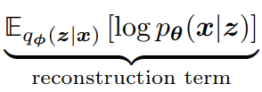
we seek to maximize this term, and therefore we do the following:

Sample some x’s from our data distribution, and compute q(z|x)
Sample from our q(z|x), compute p(x|z)
Take the gradients, and try to maximize, repeat

This is effectively an estimate of maximizing the distribution p(x|z) through the expectation of q(z|x), because we have many samples of x which we compute q(z|x) with, and then sampling from this distribution, we approximate how well q(z|x) is maximizing the likelihood p(x|z).

Hierarchical VAE’s

In our previous problem with VAEs, we modeled how a latent variable ‘z’ generated a higher-dimensional projection ‘x’. Hierarchical VAEs are a generalization, where we can have multiple latent variables z1,z2… and each latent can be a lower-dimensional projection of another.

In our case, we will focus on the Markov case where each z_n only depends on the last latent-variable.

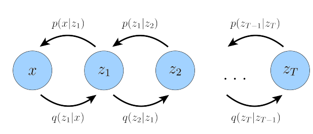
Using this markov-chain property, we can rewrite the joint distribution, and the posterior distribution as:

We can plug this equation into the ELBO similarly as we did before, and obtain the same formula for it:

and then notice we plug in our new formulation for our joint and posterior. This makes sense, because our ELBO is effectively just telling us that when introducing a surrogate to try to reconstruct the loss, this is what we must maximize the maximize how close we are to the true evidence; no matter how many variables are involved.

Variational Diffusion Models

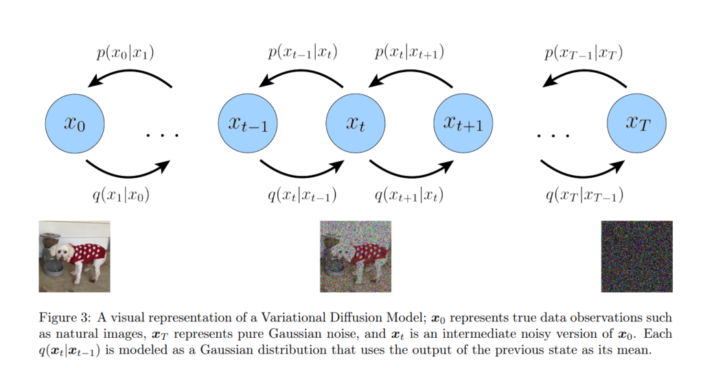
A variational diffusion model is simply an HVAE with some caviats:

Each q that decodes a previous timestep has fixed parameters (Gaussian centered around previous timestep output)
The dimensionality of each latent variable is the same
The final latent-encoding z_T is pure gaussian noise

Here is a visual representation, with a hint to why we are setting these restrictions for our model:

Here is formally how we denote each q_t:

Basically, since we can change α at each level, we are just ensuring that the variance stays at a similar scale. The tradeoff is: at low α, we adhere less to the previous mean, and at high α, we basically barely introduce noise.

An important property of this, is that at the final timestep T (after many iterations), we converge to a normal distribution:

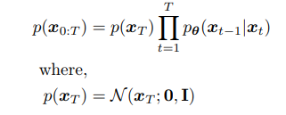
Where the first term in the integral converges to a normal distribution with mean zero, and standard deviation 1!

I understand this by saying, we basically scale down our mean by the square root of α, and then add-back in some noise to compensate for this (1-sqrt(α) standard deviation). So, over time, we have more noise that has been added, and a smaller proportion of the mean; and because we scale up our standard deviation closer to 1, and scale down our mean proportional to this (meaning we’ll always have variance of 1) we achieve a standard gaussian.

Now we are only interested in learning our p distribution parameterized by θ, which defines how our image is de-noised. If we could do this, we could simulate novel data from pure-noised images; sampling from the true image-distribution. To summarize:

We noise our images and obtain random gaussian noise
We try to learn the de-noising process in order to model the true distribution of images
Since we go step-by-step, our samples should be consistent as we re-build them when sampling from the model.

In our vanilla VAE we tried to infer the latent from an image, now we are trying to infer an image from our first latent that is normally distributed (and maximize the likelihood).

Now, let’s derive the ELBO with our new equation and see what it reveals about how we can optimize our diffusion process:

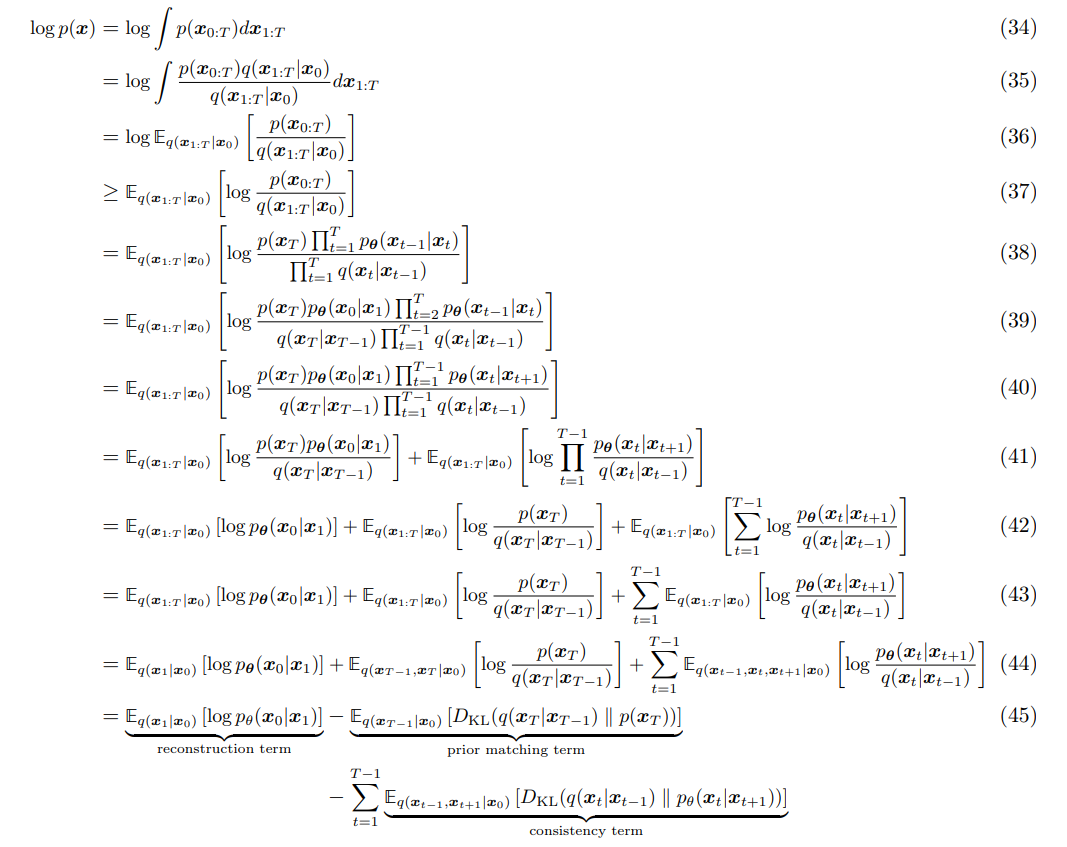
Basically, we just plug in our surrogate distribution as before, and then substitute in our equation to try to get an understanding of the properties of our ELBO, and break it down into tasks.

We get a reconstruction term, which says how we rebuild with p, given how we have defined q(x_1|x_0). This is basically the same term as our vanilla VAE
This term cannot be changed because there are no parameters. It is minimized when our final noising step matches a normal distribution (which we assume it does)
This term describes how each one of our noising steps, and denoising steps should match eachothers’ distributions. This is because the ‘true’ solution takes this into account while denoising. In this way it can be seen as similar to ‘prior matching’.

We are essentially finding the ELBO for a generalized VAE in the form of a markov chain, and it tells us that we must match p’s and q’s distribution at all steps in order to achieve approximate evidence that is close to the true evidence.

I like to think of it this way: the ELBO term in (37) tells us we need to maximize the likelihood of the joint p for a given q in order for our distributions to be ‘close’ to the ground truth. And when finding the final three terms, we are just breaking this down further to see what individual parts of p we can maximize with q (to derive a more clear objective).

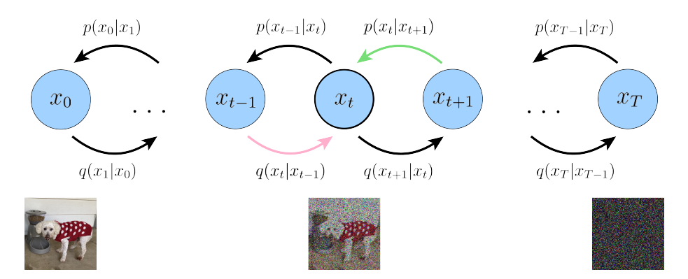
As we can see, we want each ‘reconstruction’ with p to match the noising distribution of q at the corresponding step.

Problem

Since each one of our ELBO terms is an expectation over q, we can approximate them by sampling from q’s distribution (monte carlo). However, in our consistency term, the expectation is over two different variables.

We would have to sample from both of these variables’ distributions
This would mean a higher variance from our samples (exponentially more samples needed for more variables)
Since we are summing up for all T the variance may be very high, or different from the actual expectation

Now, using some more manipulation of our formulas, and using Bayes rule, we can arrive at another ELBO that is tractable with our estimates:

This is equivalent to our last ELBO, but is much more usable:

We have our previous reconstruction term
We have a similar ‘prior-matching’ term
Our ‘Denoising-matching’ for the KL divergence between the posterior of q, and our p denoising term, which is inside the expectation of q of the previous step.

This formula is related to our vanilla VAE, as if T=1, we would achieve the same ELBO as for our VAE with one latent!

I think of this as: we are looking to maximize the following:

and this is simply maximizing the distributions of all p’s with our q distribution, or maximizing their ‘alignment’. Since we can’t do this directly, we break it up into individual components and maximize this instead. And again, the ground truth automatically would maximize this since the KL term we do not see would not exist.

And, luckily we yield our final ELBO which is easy to work with and gives us a way to do MC sampling, and have a analytical solution to the KL terms.

Denoising matching terms

Let’s focus back in on our formula:

our first term we’ve already delt with, and our second term is automatically handled. However, our third term is novel and we can treat it as follows: approximating our ‘ground-truth’ posterior q with a distribution ‘p’. Even though we treat our evidence as p this is ok, because maximizing the ELBO will still maximize our evidence.

Since the expectation distribution of q is fixed, we focus on minimizing the KL divergence between our approximate denoising step p, and our q term, which can be rewritten as:

and from sampled noise, we can model each q(x_t) as:

we can rewrite this as follows:

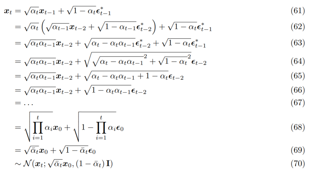
Note that we have two sets of noise we sample from, and in (64) we use the property of adding two gaussian variables.

Now that we have the Gaussian parameterization for any step in our chain, we can calculate our posterior distribution for any q:

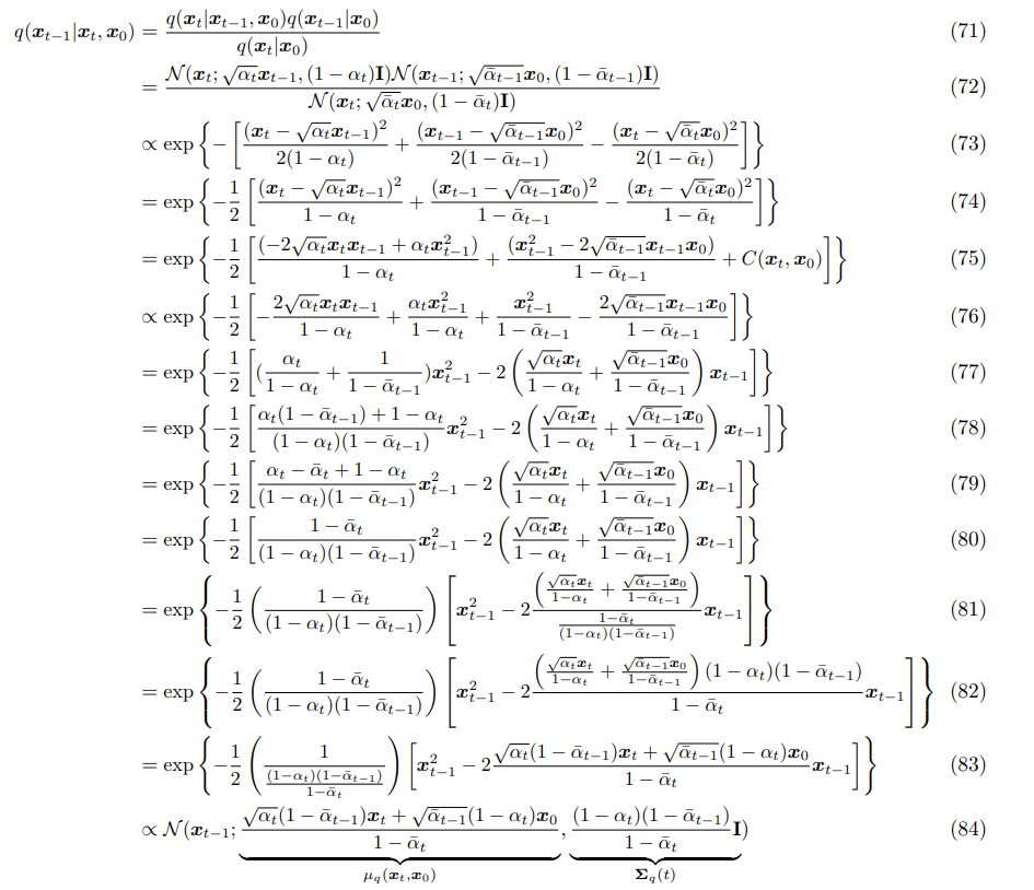
Now, although we can model our posterior in closed-form, we still need a distribution that serves for reconstructing our evidence (p), and we can used this closed-form to guide us.

We know the variance, and can parameterize our generative model p_θ with this automatically. However, the mean of our distribution is unknown (because p does not have access to x_0), and we will approximate this with a neural network.

Although in a different form, this objective makes intuitive sense:

Our ELBO told us that to maximize our evidence, we must maximize the reconstruction at each step
This means we must learn reconstruct our noised image (mean vector) only given the timestep, and the previous noise.
With this, we would be able to generate new images from pure noise!

Now, let’s get a loss function we can use.

The KL between our two distributions is as follows:

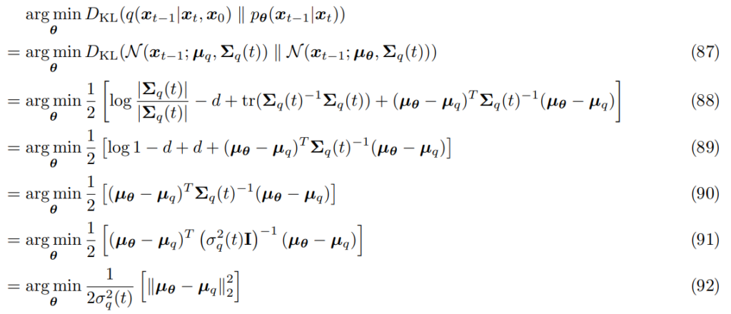
this makes sense, it is just the distance between our means scaled inversely with the variance (because more variance means a wider variety of possibilities).

Given this objective, and that we know what our μ_q is we can write our μ_θ as this:

So, we have taken our KL divergence term, and given the useful properties of gaussian distributions, isolated a single thing that we need to predict (x_0).

Here is our new problem:

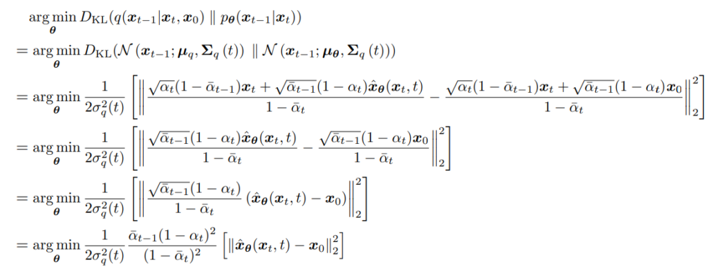
intuitively, we are just minimizing the mean squared error between our predicted x_0, and the ground truth x_0 (scaled by the variance, and some parameters).

We can approximate minimizing this by choosing random timesteps, and minimizing the deconstruction loss, mathematically:

now, we have a direct way to maximize the ELBO! We simply sample arbitrary timesteps with some noise, try to reconstruct them with an expressive neural network, and then preform gradient descent to approximate our parameters.

Noise Parameters

Although we can fix the noise parameters α, learning them may lead better results, as noising to quickly or too slowly could result in poor performance. If we expand our derived formula from above:

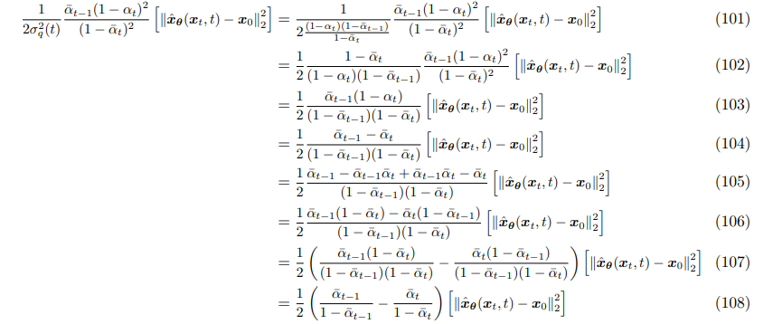
we derive the equation to be µ^2/σ^2 for t and t-1. This is important because this is the definition of signal-to-noise ratio (SNR), or the proportion of meaningful input to noise. A larger mean is interpreted as knowing more about the data, while a large variance reveals uncertainty. The reason a larger mean means more signal, is because we assume our image to start with values away from zero, and they slowly converge to zero over time (and gain larger variances).

So, we can write our KL loss as:

I think of this as: if we are dealing with larger amounts of noise in our current distribution (larger SNR), and smaller amounts of noise in our target distribution, our job is much harder, and therefore the loss (KL term) inherently lower by default (there’s only so much we can do with noise).

Also note that our SNR monotonically decreases, as we want to gradually add more noise to our image. Given that we want it to monotonically decrease with time, and the fact that it affects our ability to reconstruct the data, we can parameterize directly our SNR as follows:

were ω_nn is a neural network that is monotonically increasing (and therefore the expression is monotonically decreasing).

We can also obtain:

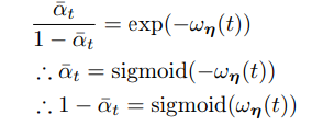
which is necessary for quick computation for arbitrary t’s.

I think of this overall as when we have more important steps (larger SNR jumps=more significant part of reconstruction), our loss is weighed more.

So, we are basically choosing a neural network (that monotonically makes the SNR decrease) that parameterizes all timesteps in order to choose strategically which noise-steps to have the most significant ‘jumps’ in noising/denoising.

Predicting noise

We know what any x_t is given x_0, so we can determine x_0 simple with:

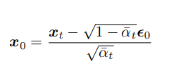
where epsilon_0 is all the noise aggregated previously. This lends to the perspective, that we can actually predict the noise eps_0, instead of x_0 directly! This makes sense, because given a noisy image, predicting what noise was added is the same as predicting the original image.

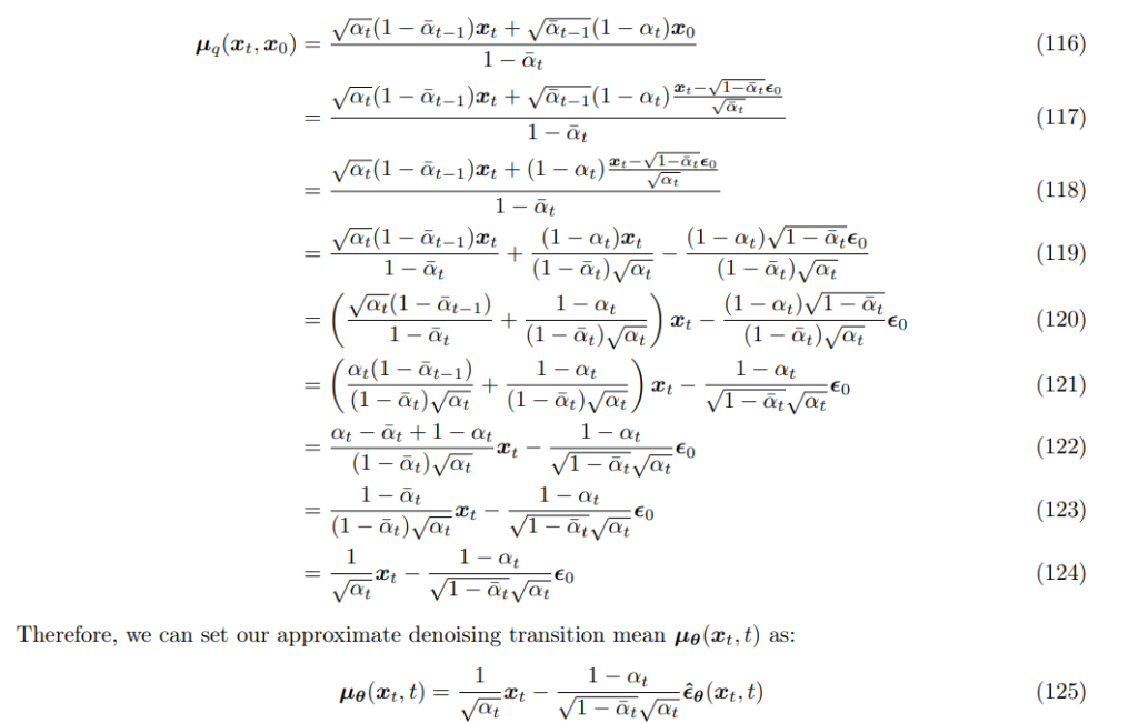
So, mathematically we can just focus on predicting the noise as an equivalent objective. We would simply then just have to plug this back into our KL divergence of two gaussians formula, and obtain:

This was a little odd to me at first, however it makes complete sense, because the reason we need a neural network to predict x_t-1 is because we do not know the original source that added the noise! Therefore, if we knew what the noise was, this is exactly equivalent to predicting the very original image.

It has also been shown in practice that predicting the noise is a better objective.

“Tweedie’s formula”

Tweedies formula basically involves a correction term when estimating the true mean of a distribution when we know the variance.

Basically, the point of this formula is to sidestep estimation of a prior (which μ is sampled from), which is unknown to us.

If we observe some data point z, we just shift it towards the mean depending on how far away we are from it, and how much variance there is. Furthermore, the ‘datapoint’ can actually be a maximum likelihood estimate. Basically this is a shortcut for Bayes rule, and a way to ‘update’ our beliefs about z given a prior p(z).

This gives us for a gaussian distribution access to the posterior mean and MAP. If we were to have more samples, we would divide the score correction term by the number of samples (because we are more certain z is correct).

Besides being a useful bias-correction tool in statistics, this reveals something interesting about our problem. When we use this to try to estimate the mean for x_t, we obtain:

and therefore, we can use our derivative of log p(x_t) in place of x_0 in what we predict. So, our KL divergence can become:

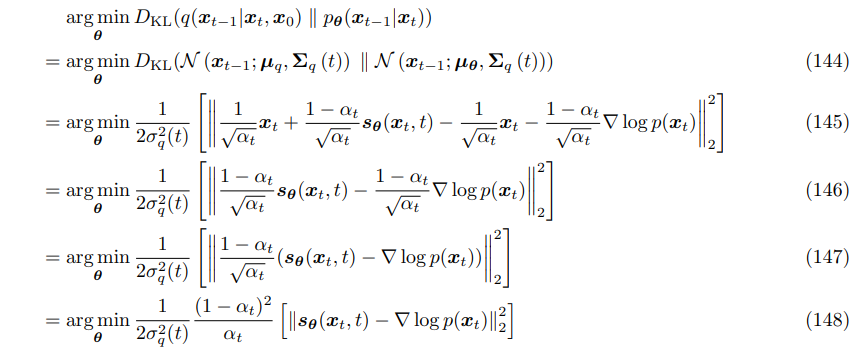
so, instead of predicting x_0, or the noise, we actually predict the derivative of the log of our next sample to obtain the denoised image.

Furthermore, this objective is actually similar to predicting the noise!

Basically, the intuition behind this is that our score function gives us the direction to move to maximize the probability of a given image. This direction is the same as moving in the opposite direction of the noise.

To recap what we’ve done so far

Extended our ELBO to our markovian HVAE in order to have a proxy objective to maximize (in order to maximize our evidence)
Define a gaussian noising process, and use it’s properties to obtain a ground-truth posterior, and define our KL divergence (when we only need to guess the mean)
Framed our problem in the equivalent perspective of predicting the noise, or the score-function, which is the direction in which the probability is increasing (and how much).

Score-based models

Score-based generative models are looked at through another perspective, however achieve an equivalent formula as our score-matching objective we previously derived.

Energy-based models

yann-tutorial

First, let’s quickly understand what an energy-based model is. Energy-based models attempt to solve the problem of predicting continuous things. Essentially, instead of having discrete outputs, we want to know how well x (input) fits with y (output). A good model will make the energy-function low for the right pair, and high for the wrong-pair.

We define a function F(x,y) that outputs the independence of x and y (high values mean diseperate), and in inference we try to minmize this function with y through gradient descent.
We learn the energy-based-model itself with gradient descent.

So, we can either preform gradient descent to learn an energy function, or to learn a given input if we are missing one and have a trained energy function.

Application

So, we have defined an energy function, now let’s relate it back to probability:

where f is our energy function and z is a normalizing constant. Say we want to ‘learn’ this distribution, we can simply try to maximize the likelihood of our samples x. However, this is intractable, as Z is not available to us. However, there is a way around this:

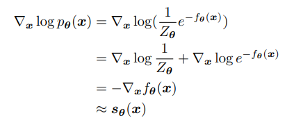
Think of this as: the ‘score function’, or direction we should move to increase probability is the same as the derivative of where to decrease our energy (when we define p(x) as above).

The score function can be visualized as a vector-field pointing to higher-density probability regions. If we learn a score-function for arbitrary points of x, we can push them towards the true distribution (noised image-> real image).

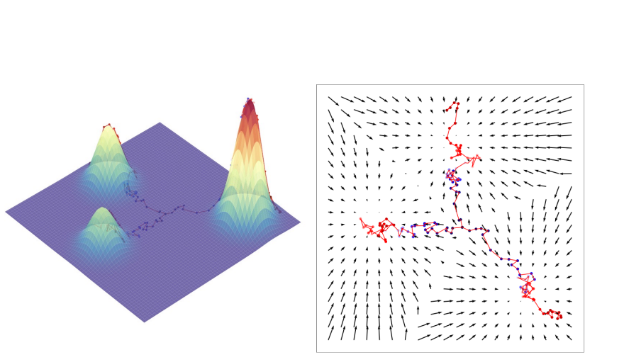
The left image can be interpreted as the derivative of our energy function, and the right, different image-samples.

Ideally, we would learn to model, for each sample, the score function that pushed our noised image towards the real image (and therefore learn the distribution of images in high-dimensional space). For example, a noised image would somewhat close to one of the distributions, and a good score function should be able to guide it closer to it’s respective distribution.

problems

CONTINUE LATER

Denoising Implicit Diffusion Models

DDIM paper

DDIM models are a deterministic version of the DDPM that have faster sampling than DDPMs, but with the same training.

Here is a high-level overview:

There is a specific parameter that allows us to determine how ‘deterministic’ our sampling will be.
The training objective is the same as DDPMS
We can sample from arbitrary steps in the diffusion denoising process (this is what stable diffusion uses)

The authors claim that not only does DDIM speed up the diffusion process compared to DDPM’s, but it actually allows for more ‘consistency’, where similar latent-variables will generate similar high-level features. This is because their deterministic nature. Furthermore, since we have a deterministic generative process, we can ‘interpolate’ in the latent-codes to produce meaningful images, rather than the DDPM model which has stochastic nature, and therefore interpolation is not possible (since the outputs would randomly change).

Math of DDPM vs. DDIM

Let’s look at the difference between our DDPM model and DDIM model in how inference is preformed. For a noising process q, we can derive the following about the log probability:

We just re-write our log probabilities based on the formula for normal distributions. Given Bayes rule, we can find the posterior distribution q(x_t | x_t-1).

Ok, so basically we’ve isolated the x_t-1 variables to define our posterior, which are all we need, since these are what we actually need to maximize. The f can be left out of the equation, because it is effectively a normalization constant that can be ignored.

So, now lets find:

in order for us to be able to derive a KL objective and parameterize with our approximate denoiser p. We need to be able to now derive the mean and variance from some exponential formula here, which we can simply do by completing the square:

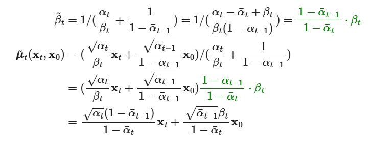
So, we’ve simply harnessed the properties of Gaussians to derive a term for the posterior mean and variance given what we know. Furthermore, for x_0 we can plug in: